SAP HANA: Analytic View

What is Analytic View?

            Analytic View is basically used to represents star models in HANA where the fact table is surrounded by different dimensions (master data). Analytic View is best suited for the scenarios where we need aggregated data from underlying tables that contain large data sets.

In SAP HANA Analytic view, dimension table is joined with the fact table that contains transaction data.

A dimension table contains descriptive data. (E.g. Product, Product Name, Vendor, customer, etc.). Fact Table contains both descriptive data and Measureable data (Amount, Tax, etc.).

SAP HANA Analytic view forms a cube-like structure, which is used for analysis of data.

Analytic views leverage the computing power of SAP HANA to calculate aggregate data, e. g., the number of bikes sold per country, or the maximum power consumed per month.

Optionally, attribute views can also be included in the analytic view definition. In this way, you can achieve an additional depth of attribute data.

You can model the following elements within an analytic view:

1.      Columns

2.      Calculated Columns

3.      Restricted Columns

4.      Variables

5.      Input Parameters

Node:

In the Semantics node, you can classify columns and calculated columns as type attributes and measures. The attributes you define in an analytic view are Local to that view. However, attributes coming from attribute views in an analytic view are Shared attributes.

You can choose to further fine-tune the behavior of the attributes and measures of an analytic view by setting the properties as follows:

·         Filters to restrict values that are selected when using the analytic view.

·         Attributes can be defined as Hidden so that they are able to be used in processes but are not viewable to end users.

·         The Drill Down Enabled property can be used to indicate if an attribute is available for further drill down when consumed.

·         Aggregation type on measures

·         Currency and Unit of Measure parameters (you can set the Measure Type property of a measure, and also in Calculated Column creation dialog, associate a measure with currency and unit of measure)

Creating an Analytic View:

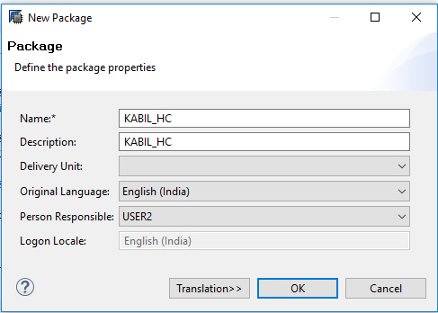
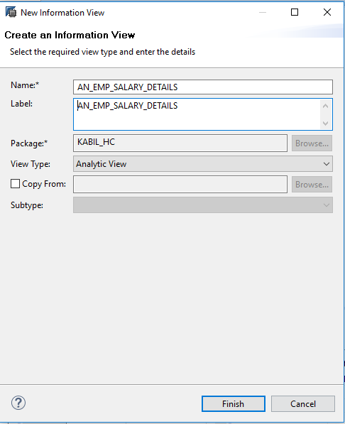
Step 1: Right-click on your package select New and select Analytic View. And Provide the details and click OK.

Step 2: Drag and Drop the required tables in a Data foundation.

Step 3: Here, I used the “TH_EMP_SALARY” Table and EMPLOYEE_DETAILS Attribute View. And make a join between them by using their relationship. Here I make a link based on “EMP_ID”.

Step 4: Click validate and Activate the view.

Step 5: Data Preview result

SAP HANA: Attribute Views

·         Attribute view acts like a dimension.It joins multiple tables and acts as Master.

·         Attribute views are built specifically for master data.

·         There is no measure and aggregation option.

·         Attribute view is reusable objects.

·         Their primary purpose was to maintain a reusable pool of master data which could then be combined with transaction data in Calculation views or Analytical views

·         It doesn’t store the data physically, however, fetches the data from a source in runtime whenever we execute this object in our system.

Creation of Attribute view:

Step 1: Create Package by right click the Content and select New and select Package

Step 2: Then we get a package creation Pop-up screen where we are required to enter its Technical name, Description, Delivery unit, Language, and Person responsible.

Click ‘OK’ after entering the details. We should then be able to see a package with the same name under our content folder. Here, I named it as “KABIL_HC”.

Step 3: Create Attribute View by right click the package “KABIL_HC” and select New and select Attribute View.

In the below screen we have to enter the details for our Attribute View, like Technical Name, Description(Label) and Type of object (Subtype). We can create three types of Attribute Views, they are

1.      Standard

2.      Time

3.      Derived

Standard: This is normal attribute view which is defined on one or multiple source tables that has already sourced in HANA.

Time: If we need to create time dimension based on time/date tables that we have in our HANA system under _SYS_BI schema, then we can choose this.

The tables are M_TIME_DIMENSION and M_FISCAL_CALENDAR.

Derived: If we want to derive a view from an existing attribute view then we need to choose this. The only editable in this type is the description of the new Attribute View.

If we want to define an attribute view by using one of our existing objects as a copy, then we can choose ‘Copy From’ option.

Note: The difference between Copy from and Derived is that in case of derived we can only edit the description of the new attribute view, all the remaining changes can only be performed on the base object. In case of Copy From we can modify our copied view entirely.

The below screen opens up. Notice that the semantics is not connected to an Aggregation node here. It is connected to a “Data Foundation”.

A “Data Foundation” is a node which you cannot remove. It is purely used to include tables into the view. You can use a singular table here or have more by specifying the join condition inside this “Data Foundation”.

You cannot insert views into the “Data Foundation”. It only accepts tables.

Step 4: Now Drag and Drop the required tables and select required fields.

Step 5: Now we are going to create a Calculated Column by right click the Calculated column and select New. A Pop-up screen will appear

Here I wrote an expression for Full name “FIRST_NAME”+’ ‘+”LAST_NAME”.

Step 6: Now Drag and Drop the “TH_EMP_MASTER” tables and select required fields.

Step 7: And the make a join link between the table with the relationship. In default, the join will be the referential join. In a property, opening up the JOIN type setting provides a list of available options. Switch it to LEFT OUTER JOIN (you can choose any type which is required for you).

Step 8: Finally, Save and activate this view. Now execute a data preview to check the data. As seen below, the JOIN is successful and data appears as required.

Result:

Thank you for visiting...

Share your comments...

SAP HANA: Introduction to Data Modeling

·         Modeling refers to an activity of refining or slicing data in database tables by creating views to depict abusiness scenario. The views can be used for reporting and decision making.

·         The modeling process involves the simulation of entities, such as customer, product, and sales, and the relationships between them. These related entities can be used in analytics applications such as SAP

·         BusinessObjects Explorer and Microsoft Office. In SAP HANA, these views are known as information views.

·         Information views use various combinations of content data (that is, non-metadata) to model a business use case.

Content data can be classified as follows:

● Attribute: Descriptive data, such as customer ID, city, and country.

● Measure: Quantifiable data, such as revenue, quantity sold and counters.

Attributes

Attributes are the non-measurable analytical elements

Attributes	Description	Example
Simple Attributes	Individual non-measurable analytical elements that are derived from the data sources.	For example, PRODUCT_ID and PRODUCT_NAME are attributes of product data source.
Calculated Attributes	Derived from one or more existing attributes or constants.	For example, deriving the full name of a customer (first name and last name), assigning a constant value to an attribute that can be used for arithmetic calculations.
Local Attributes	Local attributes that you use in an analytic view allow you to customize the behaviour of an attribute for only that view.	For example, if an analytic view or a calculation view includes an attribute view as an underlying data source, then the analytic view inherits the behaviour of the attributes from the attribute view

Measures

Measures are measurable analytical elements. That are derived from analytic and calculation views.

Measures	Description	Examples
Simple Measures	A simple measure is a measurable analytical element that is derived from the data foundation.	For example, PROFIT.
Calculated Measures	Calculated measures are defined based on a combination of data from other data sources, arithmetic operators, constants, and functions.	For example, you can use calculated measures to calculate the net profit from revenue and operational cost.
Restricted Measures	Restricted measures or restricted columns are used to filter attribute values based on the user-defined rules.	For example, you can choose to restrict the value for the REVENUE column only for REGION = APJ, and YEAR = 2012.
Counters	Counters add a new measure to the calculation view definition to count the distinct occurrences of an attribute.	For example, to count how many times product appears and use this value for reporting purposes.

You can model entities in SAP HANA using the Modeler perspective, which includes graphical data modelling tools that allow you to create and edit data models (content models) and stored procedures.

With these tools, you can also create analytic privileges that govern the access to the models, and decision tables to model related business rules in a tabular format for decision automation.

You can create the following types of information views:

● Attribute Views

● Analytic Views

● Calculation Views

Supported Object Types

In SAP HANA Modeler perspective, the SAP HANA Systems view lists both the active and inactive objects available in default workspace.

SAP HANA Modeler perspective supports the below object types:

● Package

● Attribute Views

● Analytic Views

● Calculation Views

● Procedures

● Analytic Privileges

● Decision Tables