What is Hierarchy?
Hierarchies help business to analyze their data in a tree structure through different levels/layers with drill-down capability. Each hierarchy comprises a set of levels having many-to-one relationships between each other and collectively these levels make up the hierarchical structure.
For example, a time hierarchy comprises of levels such as Fiscal Year, Fiscal Quarter, Fiscal Month, and so on.
We can create two types of hierarchies in SAP HANA, they are
1. Level Hierarchy
2. Parent-Child Hierarchy
Level Hierarchy:
In level hierarchies, each level represents a position in the hierarchy. For example, a time dimension can have a hierarchy that represents data at the month, quarter, and year levels.
Context
Level hierarchies consist of one or more levels of aggregation. Attributes roll up to the next higher level in a many-to-one relationship and members at this higher level roll up into the next higher level, and so on until they reach the highest level.
A hierarchy typically comprises of several levels, and you can include a single level in more than one hierarchy. A level hierarchy is rigid in nature, and you can access the root and child node in a defined order only.
Use Case:
Customer wants to analyze the sales revenue by customer country, state, and city. Now we will create a level hierarchy in our attribute view and access that using ‘MS Excel’ to analyze the sales revenue.
Example:
Here I’m going to analyze the sales amount by Country.
To create an Attribute View:
Step 1: As we already know how to create attribute view. Simply Right Click your package and select Attribute View. A pop-up window will appear and provide the details and click ok. Here I named it as “AT_CUSTOMER_GEOGRAPHY”
Step 2: Drag and Drop the required tables in a “Data Foundation” and make the link between them based on a relationship. Here, I used two tables “Dim_Customer” and “Dim_Geograpghy”. And join it by using “Geography_Key” field.

Step 3: And now we create Level Hierarchy based on Geography location like country, state, city. To Create a Hierarchy, Click Semantics, from the Details pane select Hierarchies. A Pop-up window will appear. And provide details as Shown as Below: and click “OK”

Step 4: Then Validate and Activate the view.
Step 5: And create another Attribute view for Products. Do the same thing which we have done the above. Here I used “Product” table alone.
To Create an Analytic View:
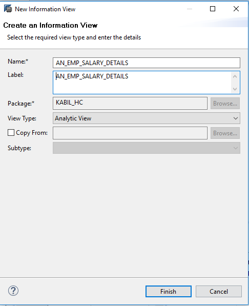
Step 1: Simply Right Click your package and select Analytic View. A pop-up window will appear and provide the details and click ok. Here I named it as “AN_ADW_FACT_INTERNET_SALES”.
Step 2: Drag and Drop the required tables in a “Data Foundation” and make the link between them based on a relationship. Here, I used two Attribute views which we are created above.
Step 3: Drag and Drop the Fact table which contains measures in another Data Foundation. Here, I used “ADW_FACT_INTERNET_SALES”. Then join this to the attributes based on the relationship.

Step 4: Then Validate and Activate the view.
Excel:
Step 1: Open Excel and Click “Data” tab and select “From Other Sources” and Choose “From Data Connection Wizard”.

Step 2: A Pop-up will appear. And choose “Other/Advanced” and Click “Next”.

Step 3: A Pop-up will appear “Data Link properties” select “SAP HANA MDX Provider” and Click Ok. A Pop-up window will appear as shown as below and provide required details. And click “ok”.

Step 4: A pop-up window will appear from this select your view which contains hierarchy. Here I choose “AN_ADW_FACT_INTERNET_SALES”. And click “Next”.

Step 5: Click “Finish”.
Step 6: Another “Import Data” pop-up will appear to select how we want to view our data from this select “Pivot table Report” and click “Ok”.

Result:
From the Pivot table Fields: select the field based on your requirement:
Here I choose following fields:
1. HI_CUS_GEO
2. OrderQuanity
3. SalesAmount

Thak you...
Share your Comments...