SAP HANA: Calculation View

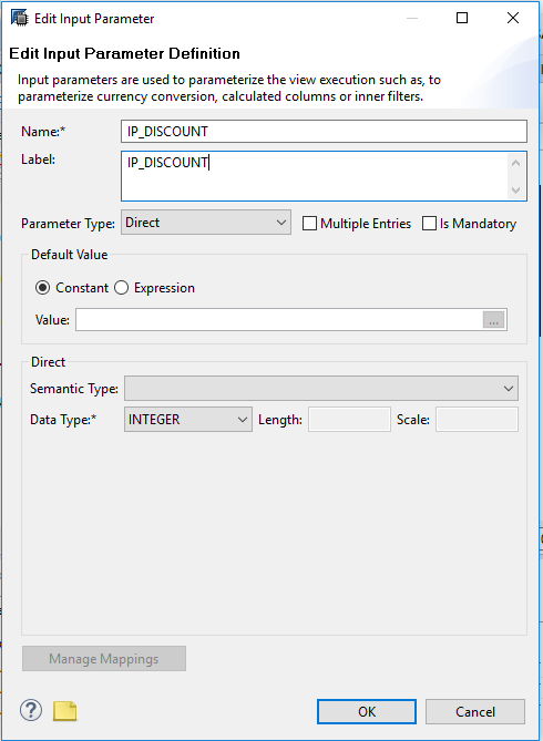
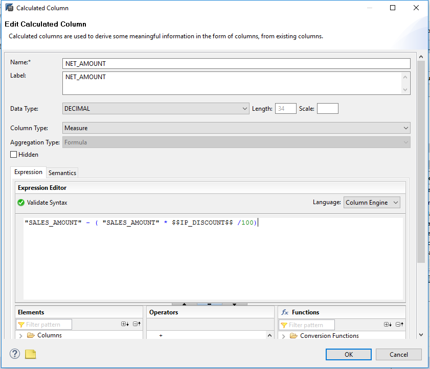
Calculation views are composite views that are used to calculate complex tabular results using either explicit SQL script code or a data flow graph that is visually created in the SAP HANA Studio.

It can consume other analytical/attribute/calculation views and tables. It can perform complex calculations that are not possible with other views.

The calculation views are of the following types:

•         Graphical calculation views are created using the graphical editor

•         Scripted calculation views are created using the SQL editor

Complex calculations, which are not possible through the graphical approach, can be created using SQL script.

Calculation views can be used in the same way as analytic views.

In contrast to analytic views, it is possible to join several fact tables in a calculation view where measures are selected from the different fact tables.

Following are general guidelines for deciding whether to use calculation views or analytic views:

•         Use analytic views where mostly aggregation of data is required. These views perform very well on database selection of data, but the opportunities for transformations are limited.

•         Use calculation views where more than one fact table needs to be combined and where complex calculations or other transformations are needed.

•         For a simple union of analytic views, the graphical method is good.

•         For complicated transformations, use the SQL method. Where possible, use the proprietary variant of the language called for, which, in this case, is SQL Script.

Graphical calculation views support the following types of calculation nodes:

Projection node

This node is used to define filters and select columns. Usually, you put each data source, such as an embedded table or view, into a projection node and apply a filter to cut down data size as early as possible.

Join node

This node is to define joins. If one table needs to join multiple tables, you need to join them one by one in separate nodes. Alternatively, you can create a star join node and then join from one table to multiple tables at one node.

With a star join, all the tables need to be wrapped into calculation views. Star joins are like analytic views except they allow you to create measures from different tables.

You can make inner joins, outer joins, referential joins, and text joins on a calculation view as well, but there is a limitation on text joins. The filter on the WHERE clause of a query will not be pushed down to the table level when there is a text join in the calculation view. If this causes performance issues, then you need to consider a different approach than using a text join.

On the join node, SAP HANA also supports the spatial join, which enables you to handle calculations between 2-D geometries performed using predicates, such as intersects, contains, and more.

Aggregation node

This node is used to define aggregation. You can define the aggregation type as SUM, MIN, MAX, or COUNT. You also can create a counter, which is used to calculate COUNT DISTINCT.

Union node

•         Unions are used to combine the result set of two or more data sources.

•         The funny fact about this UNION node here is that it doesn't work like a UNION.

•         It works as a UNION ALL operator.

•         This means that keeps piling one data set below the next without aggregating them.

Rank node

With a rank node, you can filter data based on rank.

This is the exact replacement for RANK function in SQL. We can define the partition and order by clause based on the requirement. You can set the SORT DIRECTION as DESCENDING (TOP N) Or ASCENDING (BOTTOM N).

The THRESHOLD field is to set the value of N. PARTITION BY COLUMN sets the columns to partition the records into multiple windows.

In each window, it returns the Top N or Bottom N records. The DYNAMIC PARTITION ELEMENTS checkbox allows you to choose the columns dynamically from the list under PARTITION BY COLUMN in case some of these columns do not exist in the query.

SAP HANA: Variables/Input Parameters

Analytic and calculation views can contain variables, that can be bound to specific attributes. When calling the view, you can send values for those variables. These variables can be used, for example, to filter the results.

Variables are bound to columns and are used for filtering using WHERE clauses. As such, they can only contain the values available in the Columns they relate to.

Important features of variables:

·         You use variables to filter data at runtime. You assign values to these variables by entering the value manually, or by selecting it from the drop-down list.

·         You can also define whether the Variable is Mandatory or if it should have a Default Value.

·         You can apply variables only in analytic and calculation views.

Variable Types:

The following types of Variables are supported:

Single Value: Use this to apply a filter to a Single Value.

Interval: Use this where you want the user to specify a set start and end to a selected Interval.

Range: Use this when you want the end user to be able to use operators such as “Greater Than” or “Less Than”.

System Tables to see Variable Information:

SAP HANA includes the following set of tables that contain information about the variables defined for views: There are 4 system tables under the schema _SYS_BI which contains information about Variables.

1.      BIMC_VARIABLE

2.      BIMC_VARIABLE_ASSIGNMENT

3.      BIMC_VARIABLE_VIEW

4.      BIMC_VARIABLE_VALUE

Input Parameters:

You use input parameters to define internal parameterization of the view to obtain the desired functionality when you run the view.

Input parameters in HANA are used to filter the data using the user input value as a source to perform additional calculations which helps to solve dynamic data population scenarios.

Difference between Variable and Input parameter:

Variable	Input Parameter
Variables are defined on attributes to filter the data based on user input during runtime	Input parameters defined to take user input during runtime and use it for data filtering or for dynamic calculations.
Variables apply filter after execution of all nodes till the semantics (at the top level)	Input parameters can apply filters at any projection level
Cannot be used as input for calculated columns and restricted columns	Can be used as input for calculated and restricted columns
It allows multiple values as input	It allows multiple values as input only at calculation view but not at analytic view level

Example:

            Here I use 3 tables named as Product, Sales_IP, Region.

Step 1: Create a Calculation view by right click the Package and click New and select Calculation View.

Step 2: A Pop-up will appear and provide details which is required and click Finish.

Step 3:  Drag a join node into the Scenario pane named as Join_1, in that drag and drop the required tables. Here I use SALES_IP and REGION. And make a link between using join based on the relationship.

Step 4:  Drag another join node into the scenario pane named as Join_2, in that drag and drop the required tables. Here I use Join_1 and REGION table. And make a link between using join based on the relationship.

Step 5: And then connect the Join_2 to the Aggregation node. Finally, it looks like as shown as below:

Step 6: Now we have to create an Input parameter, from the output pane, right-click the Input parameter and click New. A Pop-up will appear and provide necessary details as shown as below and click ok.

Step 7: Now we have to create a calculated column to know the Net amount which is discounted amount from the Sales Amount. From the output pane, right-click the calculated column and click New. A Pop-up will appear and provide necessary details as shown as below and click ok.Here I used that input parameter in an expression.

Step 8: Then now create a variable to filter the region. From the details pane, click Parameters/Variables tab and click create an icon. A pop-up will appear and provide necessary details as shown as below:

Step 9: Click ok and validate and Activate the view.

Step 10: Result

            When we click data preview a pop-up will appear to give a value for variable and input parameter as shown as below:

SAP HANA: Parent-Child Hierarchy

Create Parent-Child Hierarchies

In parent-child hierarchies, you use a parent attribute that determines the relationship among the view attributes. Parent-child hierarchies have elements of the same type and do not contain named levels.

Context

Parent-child hierarchies are value-based hierarchies, and you create a parent-child hierarchy from a single parent attribute. You can also define multiple parent-child pairs to support the compound node IDs.

For example, you can create a compound parent-child hierarchy that uniquely identifies cost centers with the following two parent-child pairs:

·         CostCenter and ParentCostCenter and

·         ControllingArea and ParentControllingArea,

A parent-child hierarchy is always based on two table columns and these columns define the hierarchical relationships amongst its elements.

Others examples of parent-child hierarchies are bill of materials hierarchy (parent and child) or employee master (employee and manager) hierarchy.

Example:

            Here I used two tables named as PC_HIER_EMP_DETAILS and PC_HIER_MANAGER to create a parent-child hierarchy.

Procedure:

Step 1: Create an Attribute view for PC_HIER_MANAGER by right click the Package and select New and choose Attribute View.

Step 2: And Provide Name and Label Details which are required and Click Finish.

Step 3: Drag and Drop the required tables and select required field.

Step 4: Click semantics and select Hierarchy tab and select Create Icon. A pop-up will appear and provide details as shown as below:

                        Hierarchy type : Parent-Child Hierarchy

                        Child Node     : Parent_Id

                        Parent Node    : Reporting_To

Step 5: Click OK. And validate and Activate the view.

Step 6: Then create an Analytic view by right click the Package and select New and choose Attribute View.

Step 7: And Provide Name and Label Details which are required and Click Finish.

Step 8: Drag and Drop the required tables and select required field. Here I used the above-created attribute view and one fact table named as PC_HIER_EMP_DETAILS.

Drag a Projection Node: Drag and Drop PC_HIER_EMP_DETAILS table and select required fields.

Star Join Node:

Step 9: And make a link between the Attribute view and the fact table in a Star Join based on their relationship. In a Semantic, hierarchy tab we can see the Hierarchy which we created in an Attribute view.

Step 10: Then validate and Activate the view.

In an Excel:

Step 1: Open Excel and Click “Data” tab and select “From Other Sources” and Choose “From Data Connection Wizard”.

Step 2: A Pop-up will appear. And choose “Other/Advanced” and Click “Next”.

Step 3: A Pop-up will appear “Data Link properties” select “SAP HANA MDX Provider” and Click Ok. A Pop-up window will appear as shown as below and provide required details. And click “Ok”.

Step 4: A pop-up window will appear from this select your view which contains hierarchy. Here I choose “AN_PC_HIER_EMP_MANAGER”. And click “Next”.

Step 5: Click “Finish”.

Step 6: Another “Import Data” pop-up will appear to select how we want to view our data from this select “Pivot table Report” and click “Ok”.

Result:

From the Pivot table Fields: select the field based on your requirement:

Here I choose following fields:

• PC_HIER_STRUCTURE
• First_Name
• Salary

SAP HANA: Counters

If you want to count the number of distinct values for one or more attribute columns, you create counters, which are a special type of columns that display the distinct count of attribute columns.

Context

You can create counters for multiple attribute columns at a time. For example, if you create a counter for two columns, then the counter displays the count of distinct combinations of both the columns.

Note

You can create counters for attribute columns in the default star join node or in the default aggregation view node only.

Example:

Consider a business scenario where you want to count the distinct products in each Product Category.

Solution:

1. Open the required information view in the view editor.

2. Choose the Star Join or the Aggregation node.

3. In the Output pane, choose the New icon drop-down.

4. Choose the New Counter menu option.

5. In the Counter dialog, provide counter name and description.

6. If you want to hide the counter for data preview, then select the Hidden checkbox.

7. In the Counters pane, choose Add.

8. In the dropdown list, choose an attribute. And it will be shown as below

9. Click Ok.

Note

            If queries on a calculation view contain filters on columns that you have not chosen to project, and if you have defined a counter on a calculation view, which you want to use in other calculation views, then you need to set the Transparent flag property to True for such columns in all nodes that contains this column and for the node in the calculation view that contains the counter. This helps counters to function at their expected behavior for the above scenario.

10. And validate and activate the view.

11. Result: In Analysis drag and drop:

Label Axis: EnglishProductCategoryName

Value Axis: Total_Product (i.e., the counter which we created)

SAP HANA: Restricted Column

Create Restricted Columns

Create restricted columns to restrict values of measures based on attribute restrictions. For example, you can choose to restrict the value for the REVENUE column only for " REGION = Australia ".

Just as the name suggests, a restricted column is a user-created column that is restricted in its output by a condition that we specify.

Context

You can apply restrictions on measures defined in the semantics node by using any of the below approaches:

1.      Apply restrictions on attribute values by using values from other attribute columns.

2.      Apply restrictions on attribute values using expressions.

Note

For restricted columns, modeler applies the aggregation type of the base column, and you can create restricted columns in the default aggregation view node or star join node only.

Example:

            Here I restrict a Sales value based on region.

Procedure

1.      Open the required Analytic view or graphical calculation view in the editor. Here I used Analytic view “AN_ADW_FACT_INTERNET_SALES”.

2.      Select the default aggregation node.

Note:

You can also create restricted columns in star join nodes.

3.      Choose the Restricted Columns tab.

4.      Choose

5.      In the General section, provide a name and description to the restricted column.

6.      In the Column dropdown list, select a measure on which you want to apply restrictions.

7.      If you want to hide the restricted column for data preview, select the Hidden checkbox.

8.      Apply restrictions using column values.

a)      You can define a condition using attribute columns to apply restrictions on the base measure.

b)      Select Columns.

c)      In the Column dropdown list, select an attribute column.

d)      In the Operator dropdown list, select a required operation to define the condition.

e)      In the Value field, select a value from the value help.

f)       If you want to apply restrictions only for the defined conditions, choose Include.

Note:

You can apply restrictions using more than one attribute column.

9.      It will be like as shown as below:

10.  Click “OK”.

11.  The output pane will be like this:

12.  And Validate and Activate the view.

13.  Result: Data Preview

Thank you...

Share your Comments...

SAP HANA: Level Hierarchy

What is Hierarchy?

Hierarchies help business to analyze their data in a tree structure through different levels/layers with drill-down capability. Each hierarchy comprises a set of levels having many-to-one relationships between each other and collectively these levels make up the hierarchical structure.

For example, a time hierarchy comprises of levels such as Fiscal Year, Fiscal Quarter, Fiscal Month, and so on.

We can create two types of hierarchies in SAP HANA, they are

1.      Level Hierarchy

2.      Parent-Child Hierarchy

Level Hierarchy:

In level hierarchies, each level represents a position in the hierarchy. For example, a time dimension can have a hierarchy that represents data at the month, quarter, and year levels.

Context

Level hierarchies consist of one or more levels of aggregation. Attributes roll up to the next higher level in a many-to-one relationship and members at this higher level roll up into the next higher level, and so on until they reach the highest level.

A hierarchy typically comprises of several levels, and you can include a single level in more than one hierarchy. A level hierarchy is rigid in nature, and you can access the root and child node in a defined order only.

Use Case:

Customer wants to analyze the sales revenue by customer country, state, and city. Now we will create a level hierarchy in our attribute view and access that using ‘MS Excel’ to analyze the sales revenue.

Example:

            Here I’m going to analyze the sales amount by Country.

To create an Attribute View:

Step 1: As we already know how to create attribute view. Simply Right Click your package and select Attribute View. A pop-up window will appear and provide the details and click ok. Here I named it as “AT_CUSTOMER_GEOGRAPHY”

Step 2: Drag and Drop the required tables in a “Data Foundation” and make the link between them based on a relationship. Here, I used two tables “Dim_Customer” and “Dim_Geograpghy”. And join it by using “Geography_Key” field.

Step 3: And now we create Level Hierarchy based on Geography location like country, state, city. To Create a Hierarchy, Click Semantics, from the Details pane select Hierarchies. A Pop-up window will appear. And provide details as Shown as Below: and click “OK”

Step 4: Then Validate and Activate the view.

Step 5: And create another Attribute view for Products. Do the same thing which we have done the above. Here I used “Product” table alone.

To Create an Analytic View:

Step 1: Simply Right Click your package and select Analytic View. A pop-up window will appear and provide the details and click ok. Here I named it as “AN_ADW_FACT_INTERNET_SALES”.

Step 2: Drag and Drop the required tables in a “Data Foundation” and make the link between them based on a relationship. Here, I used two Attribute views which we are created above.

Step 3: Drag and Drop the Fact table which contains measures in another Data Foundation. Here, I used “ADW_FACT_INTERNET_SALES”. Then join this to the attributes based on the relationship.

Step 4: Then Validate and Activate the view.

Excel:

Step 1: Open Excel and Click “Data” tab and select “From Other Sources” and Choose “From Data Connection Wizard”. 

Step 2: A Pop-up will appear. And choose “Other/Advanced” and Click “Next”.

Step 3: A Pop-up will appear “Data Link properties” select “SAP HANA MDX Provider” and Click Ok. A Pop-up window will appear as shown as below and provide required details. And click “ok”.

Step 4: A pop-up window will appear from this select your view which contains hierarchy. Here I choose “AN_ADW_FACT_INTERNET_SALES”. And click “Next”.

Step 5: Click “Finish”.

Step 6: Another “Import Data” pop-up will appear to select how we want to view our data from this select “Pivot table Report” and click “Ok”.

Result:

From the Pivot table Fields: select the field based on your requirement:

Here I choose following fields:

1.      HI_CUS_GEO

2.      OrderQuanity

3.      SalesAmount

Thak you...

Share your Comments...